Wassersound: morphing sound by moving mass
A 2020 side project with my friend Armand on audio and optimal transport
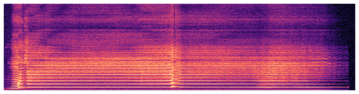 A shakuhachi spectrogram later used for morphing.
I’m teaching for the first time in ages this Fall! The class is a graduate seminar course on distribution matching and morphing. While figuring out a few fun applications of computational optimal transport, I was sent back to a pandemic project (6 years ago!) with my friend Armand Bernardi. Armand had been long thinking about algorithmic and digital approaches to music composition. I was intrigued about a (then) recent paper of Geoffrey Schiebinger describing a quantitative theory of cellular development based on optimal transport. We explored how optimal transport could be used as a subroutine for algorithmic sound effect generation, playing around with existing work I refer to throughout the blog post.
I loved working on this project so decided to talk about it here. On top of learning from Armand about algorithmic music generation, and having a fun few days hacking, this project ended up matching a pattern. Many real-world problems can be modeled with elegant mathematical formalism, but the real-world details are most often messy and the hardest to crack.
Wassersound
A simple and natural place to start is a glissando. Think of a violin dramatically joining two notes together pulling the string in the right way – got it? Optimal transport is a mathematical framework that can play the role of the violinist’s fingers, and continuously morph one sound into another. Specifically, each sound sample is spectrum over frequencies (e.g., the representation of the sound wave in Fourier space), and OT will tell you how to map frequency bins from one sound to another, directly enabling morphing.
For this article, I recorded two samples on the shakuhachi, a japanese bamboo flute I study (perhaps the topic of a later post!):
Source A — Tsu Re:
Source B — Ro Chi Re Chi:
Morphing by amplitude
Linearly interpolating two raw audio waveforms — represented by an amplitude over time — just crossfades them. Metaphorically, that’s what your cousin DJ-ing at a birthday party and transitioning between soundtracks would do. Let’s listen to it.
As expected, during the transition period, we get superposition of the two tracks, and at the midpoint both notes are audible simultaneously. Therefore, you perceive a chord rather than a single pitch in transition. What would be musically more appealing is a signal that, at the midpoint, sounds like one note whose pitch lies between A’s and B’s. That is a statement about interpolating distributions of spectral energy, not about interpolating waveforms.
Moving into Fourier space
Our next move is therefore to go to the frequency domain. We use a short-time Fourier transform (STFT): slide a 50 ms Hann window across each source in steps of half a window, and take an FFT at each position. The result is a complex spectrogram $S \in \mathbb{C}^{T \times N}$, with $T$ time-frames along the horizontal axis and $N$ positive-frequency bins along the vertical (we use a 50 ms window with 8× zero-padding, but the exact bin count doesn’t matter for what follows). Each column $S_{t.}$ is a snapshot of which frequencies are present, at what amplitude and phase, during frame $t$.
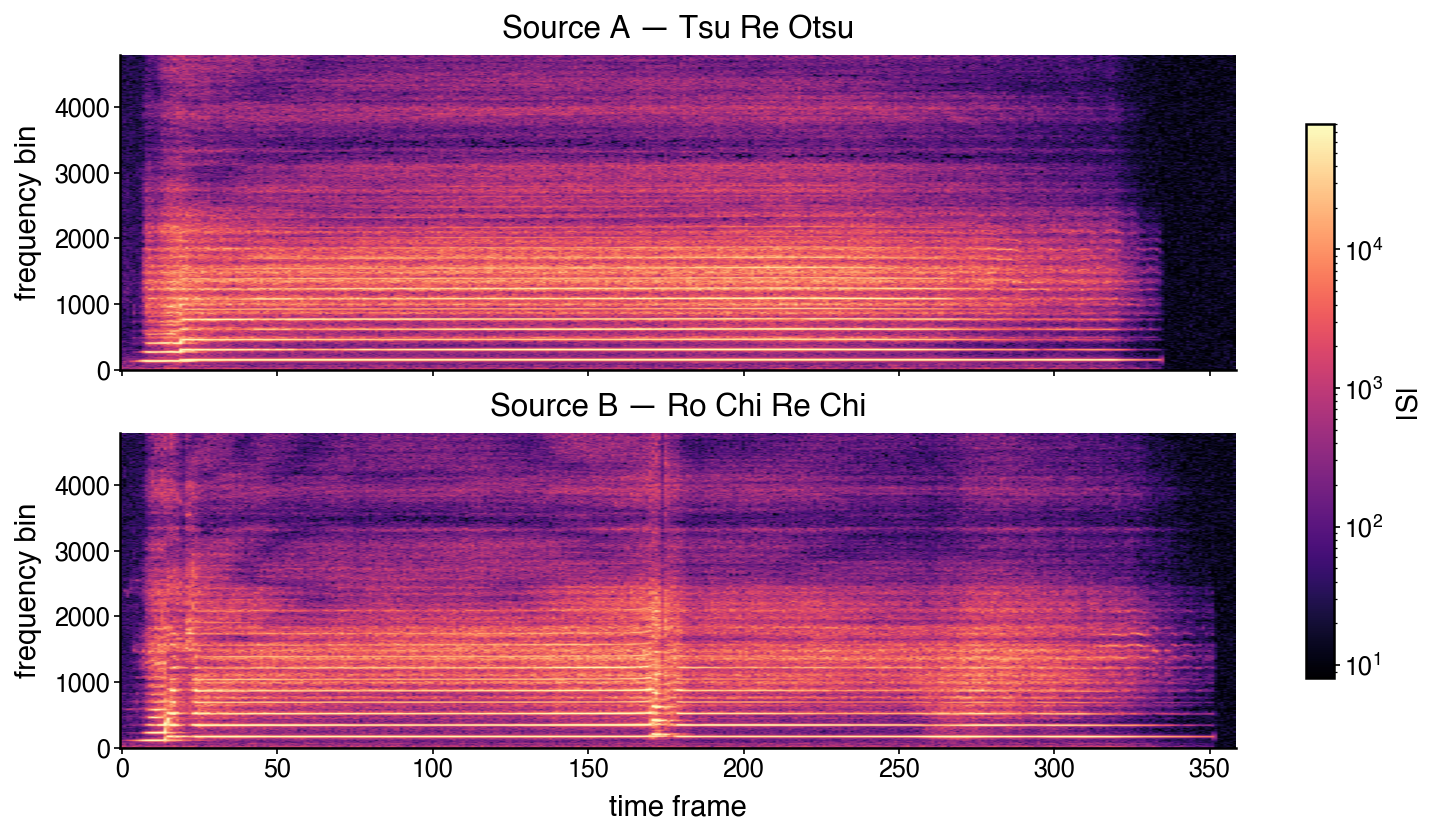
Both sources are shakuhachi notes with roughly stationary timbre: you can see clean horizontal bands corresponding to a fundamental and its harmonics, fairly stable in time but at different frequencies for A and B. This is exactly the kind of signal where frame-by-frame magnitude spectra are meaningful objects, and where morphing them by moving mass along the frequency axis has a clean physical interpretation.
We then turn each frame $S_{t.}$ of the audio sample into a probability distribution over frequency $p_{t.}$:
$$ p_{t,k} = \frac{|S_{tk}|}{\sum_{k'} |S_{tk'}|}. $$
At each of the $T$ time-frames, we now have $N$-dimensional probability vectors, $p_t^A$ and $p_t^B$ for each audio signal $A$ and $B$. The morphing problem reduces to: for each $t$, interpolate between $p_t^A$ and $p_t^B$ using optimal transport.
Optimal transport and cost functions
Given two discrete distributions $\mu^0$ and $\mu^1$ on a shared ground space (here, our frequency bins) and a cost $C_{ij}$ for moving a unit of mass from bin $i$ to bin $j$, optimal transport finds the transport plan $\pi \in \mathbb{R}_+^{N \times N}$ that minimises
$$ \langle C, \pi \rangle = \sum_{i, j} C_{ij}\pi_{ij}, $$
subject to the positivity constraints for $\pi$, as well as the following marginal constraints
$$\pi \cdot \mathbb{1} = \mu^0,$$
and $$ \pi^\top \mathbb{1} = \mu^1. $$ Those constraints force $\pi$ to be a valid coupling of $\mu_0$ and $\mu_1$. We are especially interested in the minimiser $\pi^*$ which we call the transport plan. This problem can be approximately solved quickly with an entropic regularisation term via the Sinkhorn algorithm.
The piece that matters for sound design is the cost matrix $C$. $C_{ij}$ is our model of “how far apart is frequency $i$ from frequency $j$?", and the answer shapes the morph. We experimented with two choices.
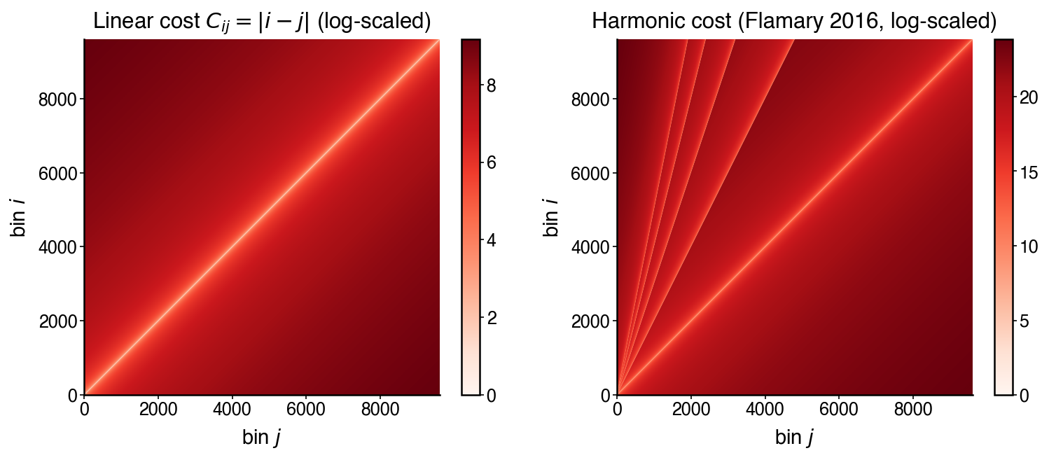
Linear cost in frequency. The simplest option: $C_{ij} = |i - j|$, normalised to $[0, 1]$. This just says that moving mass between nearby frequency bins is cheap and across the spectrum is expensive.
Harmonic cost. A musically smarter choice, borrowed from Flamary et al. (2016). A note at fundamental $f$ and a note at $2f, 3f, \ldots$ are perceptually related — they are partials of the same harmonic series. So moving mass from $f_i$ to a harmonic multiple of $f_j$ should be almost as cheap as moving it to $f_j$ itself:
$$ C_{ij}^{\text{harm}} = \min\left( (f_i - f_j)^2, ; \min_{q \in [2, Q]} (f_i - q f_j)^2 + \varepsilon q \right). $$
The barrier term $\varepsilon q$ keeps the procedure well-defined by penalising higher harmonics slightly (we use $\varepsilon = 10$, $Q = 5$). The resulting cost matrix has a striking geometry: a main diagonal, plus secondary “rails” at $j = i/2, i/3, \ldots$ along which transport is almost free.
We will listen to both at the end of this blog post!
The last piece of machinery we need is the McCann interpolant $\mu^\lambda$ between $\mu^0$ and $\mu^1$ at parameter $\lambda \in ]0, 1[$ — a barycenter in Wasserstein space from $\mu^0$ at $\lambda = 0$ to $\mu^1$ at $\lambda = 1$. For discrete measures on a bin grid with optimal plan $\pi^\star$, it has a clean closed form:
$$ \mu^\lambda_m = \sum_{i=1}^N\sum_{j=1}^N \pi^\star_{ij} \cdot \mathbb{1}_{m = \lfloor (1-\lambda) i + \lambda j \rceil}, $$ where $\lfloor \cdot \rceil$ denotes rounding to the nearest integer. This is one appealing reason to use OT for morphing: it provides a principled continuous path from one distribution to the other.
Spectrogram Morphing with OT
To morph between sounds A and B, we compute the spectrogram $q \in \mathbb{R}^{T \times N}$ by putting the pieces together. For each time-frame $t$, we define $q_t$ as:
- Compute the OT plan $\pi^{\star,(t)}$ between $p_t^A$ and $p_t^B$
- Form the McCann interpolant for $\pi^{\star,(t)}$ at parameter $\lambda_t = t/T$
- Record $q_t = \mu^{\lambda_t}$ defined above
Look at the results:
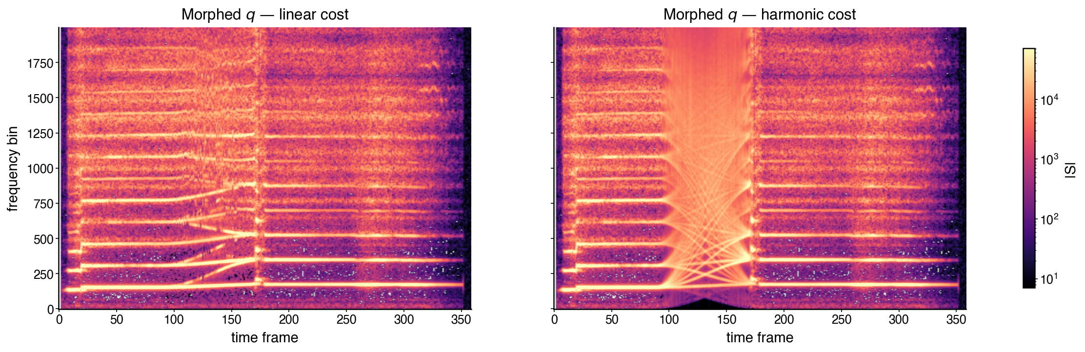
For the linear cost, the harmonic bands drift smoothly from $A$’s frequencies to $B$’s across the horizontal axis, and each individual frame looks like a plausible spectrum. For the harmonic cost, we see many crossing patterns that emerge from allowing the harmonics to match even at higher frequencies!
Reality catches up – “Where is the phase?”
Alright, how does it sound? Well, the catch is that a magnitude spectrum is not enough to reconstruct an audio signal — we also need the phase.
The cheapest (and wrong) thing one can do is to copy the phase $\arg S^A_{tk}$ from source $A$ and reconstruct the interpolation spectrogram $I \in \mathbb{C}^{T \times N}$:
$$ I_{tk} = q_{t,k} e^{i \arg S^A_{tk}}. $$
Then take an inverse FFT of each frame, overlap-add, render to a WAV. For the linear OT map, the reconstructed signal sounds like this:
Hmm, not great right? Somehow, the pitch interpolated by OT does seem to move properly, but the signal is smeared and warbling. Across consecutive frames the phase is no longer evolving coherently with the spectrum it is attached to, and the ear is extremely sensitive to that mismatch.
It was at this point we did a literature search with Armand, and discovered this really nice paper. They got this exact setup working with a few tricks based on phase accumulation, and have some demos on soundcloud worth listening. I would mention that horizontal incoherence is a hard problem. Their samples, and ours after reimplementation of their C++ code in python, are far from perfect.
Phase Reconstruction
The way out begins with noticing that we are not actually trying to recover the phase of a “true” signal — there is no ground-truth waveform whose magnitude spectrogram is $q$. What we want is some signal $x$ whose STFT magnitude is close to $q$ and that is consistent with overlap-add reconstruction. This is exactly the problem Griffin and Lim (1984) formulated forty years ago:
$$ x^\star = \arg\min_x \big| ,|\text{STFT}(x)| - q, \big|_F^2. $$
Their algorithm alternates two steps until convergence: starting from a random phase, take the inverse STFT to obtain a candidate signal, recompute its STFT, replace the magnitude by the target $q$ while keeping the recomputed phase, and repeat. The objective is monotonically non-increasing and converges to a local minimum.
This is the right relaxation for our morph: instead of borrowing phase from a signal whose magnitude is no longer there, we solve a phase-consistency problem directly on the synthesised target. The same approach was recently used in this paper on OT for music. Listen to the final results!
Linear cost with Griffin–Lim phase reconstruction :
Harmonic cost with Griffin–Lim phase reconstruction:
Conclusion
That’s it for today. Six years after, what I remember most about this fun project is how hard it was to get the infrastructure around it right (audio encoding and import, FFT, and of course phase reconstruction). It was frustrating to spend hours with Armand wondering how spectrograms that look so beautiful on the screen could sound so bad on speakers.
This small project may be good allegory for a research project. The clean equations are usually the easy part; the work that decides whether anything functions is in the seams between them — the data, the encoding, the post-processing. Building solid tools and codebases, learning the details of data processing and relating them to the reality of experiments, and checking with simple examples whether an algorithm has the expected output: these are the skills that compound across years of research and let you prototype quickly. Now back to teaching!
Acknowledgments
Thanks to Armand Bernardi for the long afternoons in 2020 listening to roughly two hundred warbling reconstructions. The reassigned-STFT analysis is a Python port of Trevor Henderson and Justin Solomon’s audio_transport, itself an implementation of Auger and Flandrin’s reassignment method. The harmonic cost is from Flamary et al. (2016); OT solvers are from POT; phase reconstruction via Griffin & Lim (1984) as implemented in librosa.
Romain Lopez
Assistant Professor of Computer Science and Biology
My research interests lie at the intersection of statistics, computation and modeling of biological data. A significant part of my research is driven by building more statistically accurate and faster machine learning software for analyzing genomics data.